ZigZag: Universal Sampling-free Uncertainty
Estimation Through Two-Step Inference*

Nikita Durasov¹, Nik Dorndorf², Hieu Le¹, Pascal Fua¹,

¹Computer Vision Laboratory, EPFL ²RWTH Aachen University

^*Transactions on Machine Learning Research 2024

Paper arXiv Code

ZigZaging. At inference time, we make two forward passes. First, we use \( [\mathbf{x}, \mathbf{0}] \) as input to produce a prediction \( \mathbf{y}_{0} \). Second, we feed \( [\mathbf{x}, \mathbf{y}_{0}] \) to the network and generate \( \mathbf{y}_{1} \). We take \( \| \mathbf{y}_{0} - \mathbf{y}_{1} \| \) to be our uncertainty estimate. In essence, the second pass performs a reconstruction in much the same way an auto-encoder does, and a high reconstruction error correlates with uncertainty.

Abstract

Whereas the ability of deep networks to produce useful predictions on many kinds of data has been amply demonstrated, estimating the reliability of these predictions remains challenging. Sampling approaches such as MC-Dropout and Deep Ensembles have emerged as the most popular ones for this purpose. Unfortunately, they require many forward passes at inference time, which slows them down. Sampling-free approaches can be faster but often suffer from other drawbacks, such as lower reliability of uncertainty estimates, difficulty of use, and limited applicability to different types of tasks and data.

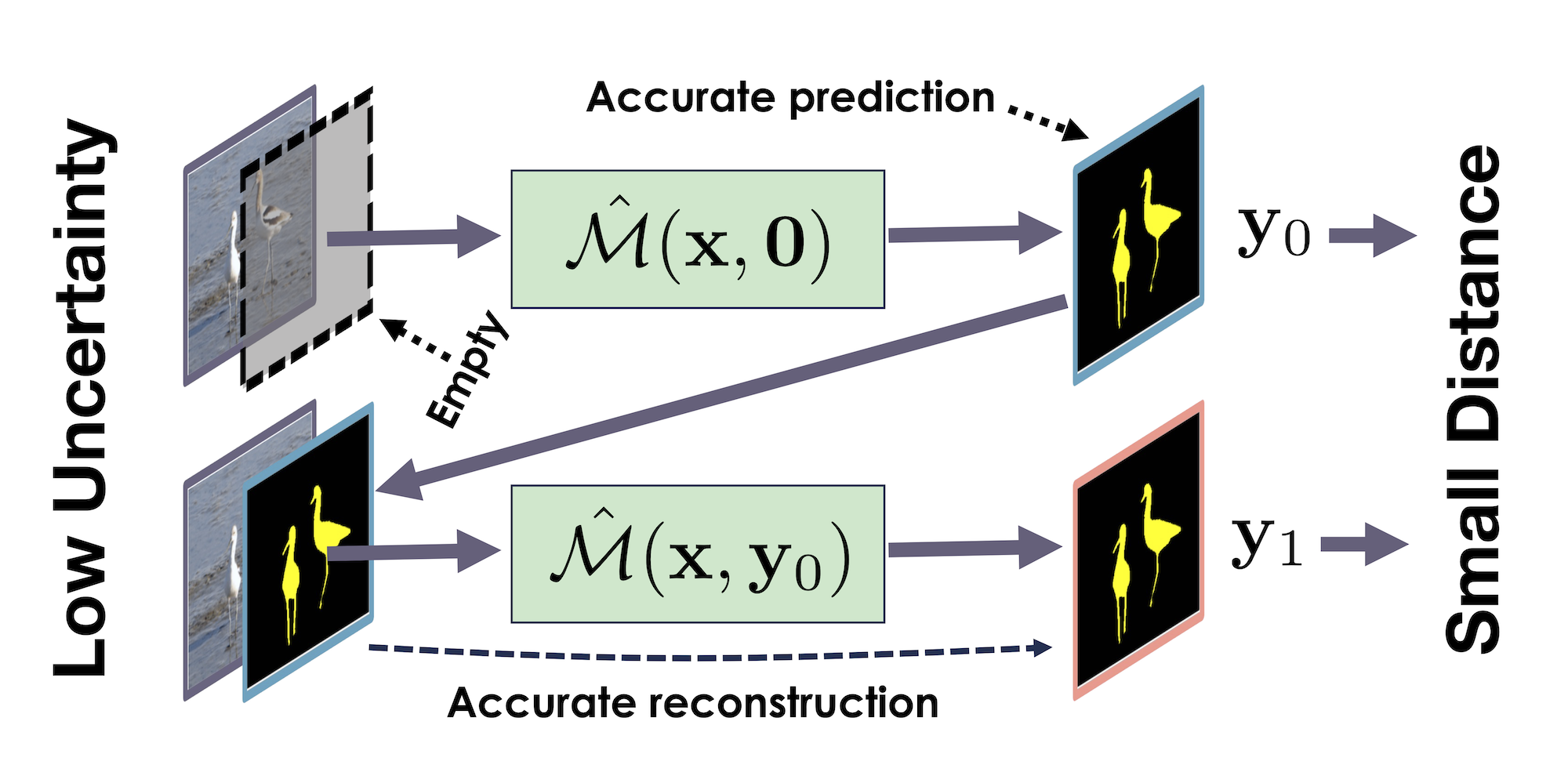
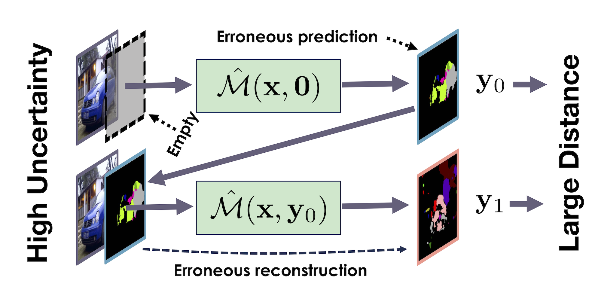
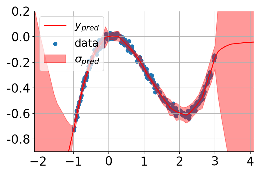
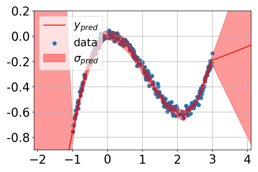
In this work, we introduce a sampling-free approach that is generic and easy to deploy, while producing reliable uncertainty estimates on par with state-of-the-art methods at a significantly lower computational cost. It is predicated on training the network to produce the same output with and without additional information about it. At inference time, when no prior information is given, we use the network's own prediction as the additional information. We then take the distance between the predictions with and without prior information as our uncertainty measure.

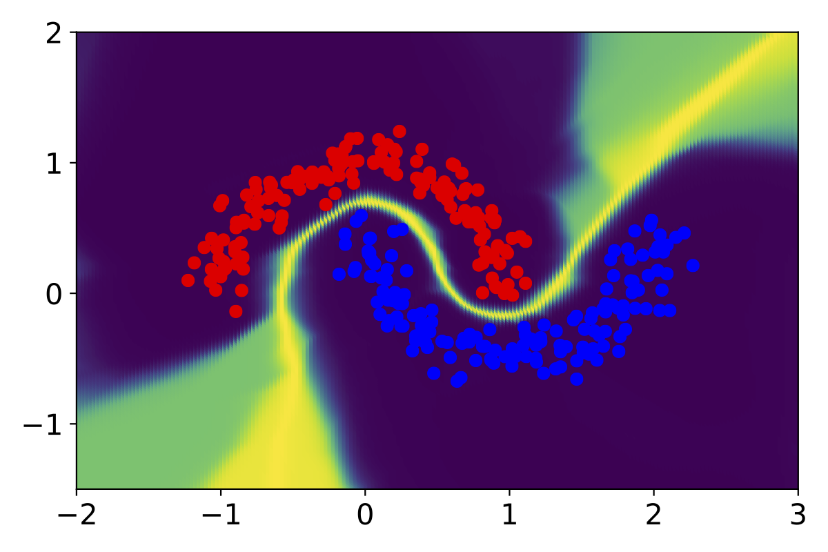
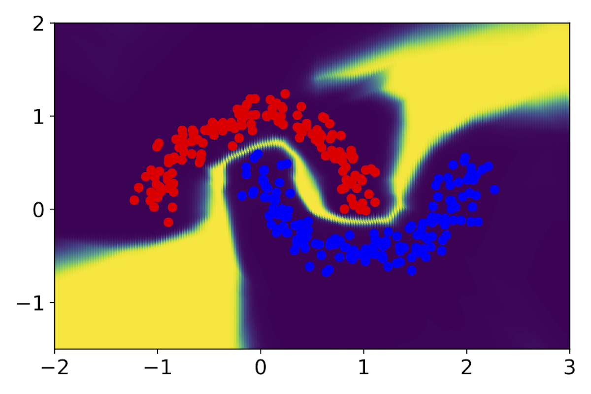
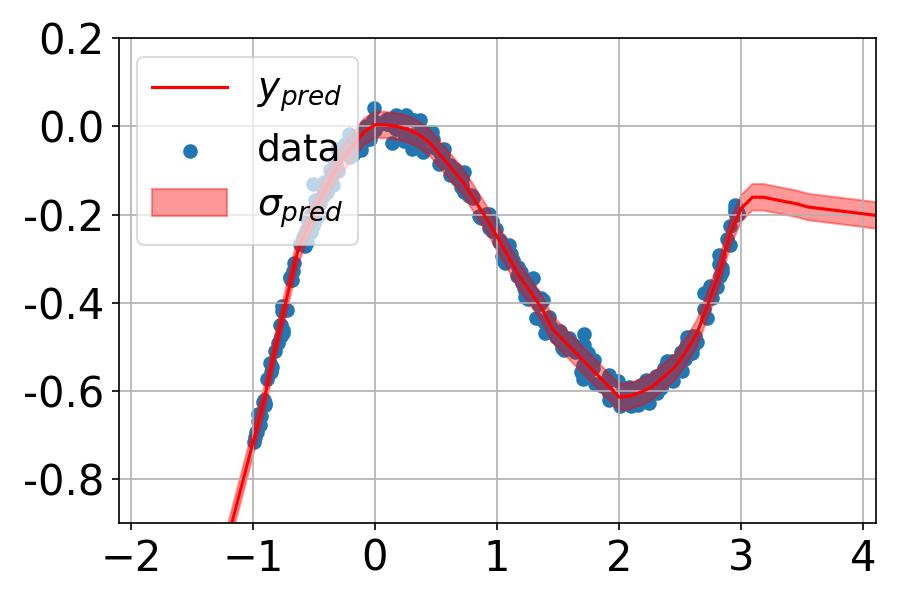
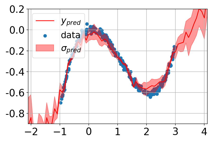
We demonstrate our approach on several classification and regression tasks. We show that it delivers results on par with those of Ensembles but at a much lower computational cost.

ZigZagging

Zigzagging involves a dual-step inference process where a neural network first generates a prediction using the initial input data. This prediction is then used as additional input in a second forward pass through the same network to generate another prediction. The disparity between these two predictions serves as the measure of uncertainty.

The method is designed to be computationally efficient, allowing for quick uncertainty assessments without the need for multiple network runs or ensemble methods, thereby facilitating faster and more resource-efficient machine learning applications.

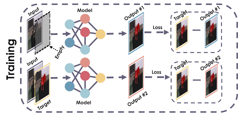
Zigzag's training scheme

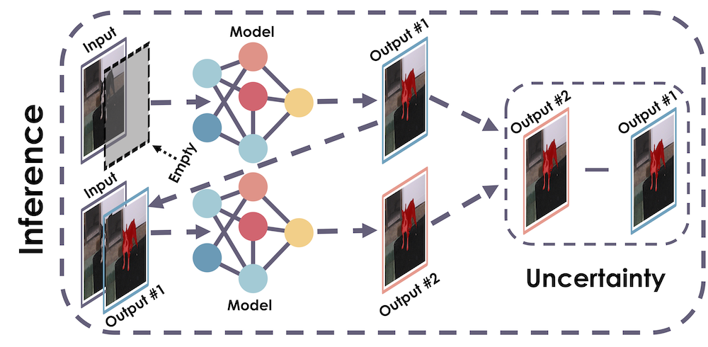
Zigzag's dual inference approach

Implementation

Integrating ZigZag into standard models is notably straightforward, requiring only minimal modifications to the first layer to accept an additional input. This simplicity enables the model to efficiently make two types of predictions—initially without and then with its own previous outputs as inputs.

ZigZag is easy to implement and meshes seamlessly with existing network architectures without extensive modifications, providing a fast and effective way to estimate uncertainty while minimizing computational demands.

Original Model

Modified Model

Motivation

The second pass reconstructs the second input, expecting lower error for in-distribution data and higher for out-of-distribution, enabling uncertainty estimation. When given a correct label \( \mathbf{y} \) with input \( \mathbf{x} \), the network, trained to minimize the difference between outputs, indicates in-distribution data. If \( \mathbf{y} \) is incorrect, this out-of-distribution sample prompts an unpredictable response, which we use to gauge uncertainty. This mechanism addresses both epistemic uncertainty when \( \mathbf{x} \) is OOD and aleatoric uncertainty when \( \mathbf{y} \) is errornous.

Results

Example 1: The task is to classify data points drawn in the range \( x \in [-2, 3] \), \( y \in [-2, 2] \) as being red or blue given the red and blue training samples from two interleaving half circles with added Gaussian noise. The background color depicts the classification uncertainty assigned by different techniques to individual grid points. Violet is low and yellow is high. (a) Single model, (b) MC-Dropout, (c) Deep Ensembles, (d) ZigZag.

Single Model

MC-Dropout

Deep Ensembles

ZigZag

Example 2: The task is to regress \( y \)-axis values for \( x \)-axis data points drawn in the range \( x \in [-1, 3] \) from a third power polynomial with added Gaussian noise. The red-colored area depicts the uncertainty assigned by different models to individual points on the \( x \)-axis grid. (a) Single model, (b) MC-Dropout, (c) Deep Ensembles, (d) ours.

Single Model

MC-Dropout

Deep Ensembles

ZigZag

Example 3: In our experiments, we evaluate ZigZag against standard baselines using the benchmark datasets MNIST vs FMNIST, CIFAR vs SVHN, and other classification and regression tasks, focusing on network training using the first dataset and performing out-of-domain detection using samples from the second. Results in Table 1 demonstrate that ZigZag and Deep Ensembles show similar performance, excelling over other methods. Notably, ZigZag achieves this without the significant increases in memory and computation overheads associated with Deep Ensembles. Despite general trends where sampling-free approaches underperform in calibration compared to sampling-based methods, ZigZag maintains robust performance. For MNIST vs FashionMNIST, we employ a standard four-layer convolutional network with ReLU activations. In CIFAR experiments, we opt for the Deep Layer Aggregation network, better suited for OOD detection in noisy, small-scale datasets like CIFAR, over traditional models like ResNet or VGG, with OOD samples drawn from non-CIFAR classes in SVHN.

Table 1: **Classification results on **MNIST** (top) and **CIFAR** (middle).** The best result in each category is in **bold** and the second best is in **bold**. Most correspond to *ZigZag* and *DeepE*. Hence, they perform similarly but ours requires far less computation and memory.
	[MC-Dropout]	[DeepE]	[BatchE]	[MaskE]	[Single]	[EDL]	[OC]	[SNGP]	[VarProb]	ZigZag	Dataset
Accuracy	0.981	0.990	0.989	0.989	0.980	0.975	0.980	0.984	0.986	0.982	MNIST
rAULC	0.932	0.958	0.941	0.929	0.712	0.955	0.851	0.813	0.731	0.961
Size	1x	5x	1.2x	1x	1x	1x	1.3x	1x	1x	1x
Inf. Time	5x	5x	5x	5x	1x	1x	1.4x	1.7x	1.2x	2x
Time	1.3x	5x	1.4x	1.3x	1x	1x	1.1x	1.1x	1.x	1x
ROC-AUC	0.953	0.984	0.965	0.963	0.773	0.947	0.934	0.951	0.812	0.982
PR-AUC	0.962	0.979	0.965	0.966	0.844	0.923	0.923	0.942	0.861	0.981
Accuracy	0.909	0.929	0.911	0.901	0.8901	0.912	0.892	0.905	0.895	0.928	CIFAR
rAULC	0.889	0.911	0.884	0.889	0.884	0.596	0.583	0.742	0.715	0.897
Size	1x	5x	1.2x	1x	1x	1x	1x	1x	1x	1x
Inf. Time	5x	5x	5x	5x	1x	1x	1.1x	1.1x	1.2x	2x
Time	1.2x	5x	1.4x	1.3x	1x	1x	1.3x	1x	1.2x	1.2x
ROC-AUC	0.854	0.915	0.877	0.900	0.825	0.864	0.851	0.900	0.831	0.901
PR-AUC	0.918	0.949	0.919	0.931	0.875	0.903	0.821	0.891	0.861	0.933

BibTeX

@article{durasov2024zigzag,
  title = {ZigZag: Universal Sampling-free Uncertainty Estimation Through Two-Step Inference},
  author = {Nikita Durasov and Nik Dorndorf and Hieu Le and Pascal Fua},
  journal = {Transactions on Machine Learning Research},
  issn = {2835-8856},
  year = {2024}
}

ZigZag: Universal Sampling-free Uncertainty Estimation Through Two-Step Inference*

Abstract

ZigZagging

Implementation

Motivation

Results

BibTeX

ZigZag: Universal Sampling-free Uncertainty
Estimation Through Two-Step Inference*